Algorithm
This explanation demonstrates calculations as SQL, but the same principles apply for other implementations.
Setup
First, I have a table that includes all utilities and subgroups. For this example I’ve create [respdata] and populated it with 100,000 records.
CREATE TABLE [respdata]
(
    [respid] int,

    -- utilities
    [sku1] float,
    [sku2] float,
    [sku3] float,
    [sku4] float,
    [sku5] float,
    [size1] float,
    [size2] float,
    [color1] float,
    [color2] float,
    [color3] float,
    [price1] float,
    [price2] float,

    -- subgroups
    [region] int,
    [gender] int,
    [group1] bit,
    [group2] bit
)
-- populate 100k records of random data
DECLARE @i int = 1;
WHILE @i <= 100000 BEGIN
    INSERT INTO [respdata]
           ([respid], [sku1], [sku2], [sku3], [sku4], [sku5], [size1], [size2], [color1], [color2], [color3], [price1], [price2], [region],          [gender],          [group1],        [group2]       )
    VALUES (@i,       rand(), rand(), rand(), rand(), rand(), rand(),  rand(),  rand(),   rand(),   rand(),   rand(),   rand(),   round(rand()*5,0), round(rand()*2,0), round(rand(),0), round(rand(),0));
    SET @i = @i + 1;
END
I'm not creating any indexes yet
Step 1: Exponeniated sum of utilities
When a user runs a forecast, a query is designed that sums the correct mix of utilities based on input configuration, per respondent.
Consider this example input configuration:

Notice in this query below that we pick only the relevant utilities (i.e. color3 for product p2) and we use only the necessary price utilities for interpolation.
WITH step1 As (
    SELECT
        *
        ,[expSumUtils.p1] = exp(sku1 + size1 + color2 + price1 + price2*0.59)
        ,[expSumUtils.p2] = exp(sku2 + size1 + color3 + price1 + price2*0.59)
        ,[expSumUtils.p3] = exp(sku3 + size1 + color1 + price1 + price2*0.19)
        ,[expSumUtils.p4] = exp(sku4 + size2 + color3 + price1)
        ,[expSumUtils.p5] = exp(sku5 + size2 + color3 + price1 + price2*0.59)
    FROM [respdata]
)
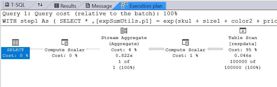
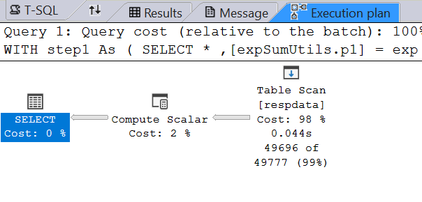
One goal is to keep the calculations at just one table scan since table scans are expensive. The query execution plan for the above uses just one table scan:
Step 2: Calculate a sum column
The share of preference calculation requires a sum of all the expSumUtils. We're naming it [expSumUtils.__sum].
The first choice calculation (not shown here) is a little different in that it calculates a max instead of a sum and finds the number of products tied at max.
,step2 AS (
    SELECT
        *
        ,[expSumUtils.__sum] =
            [expSumUtils.p1] +
            [expSumUtils.p2] +
            [expSumUtils.p3] +
            [expSumUtils.p4] +
            [expSumUtils.p5]
    FROM step1
)
SQL Server optimizes the Common Table Expressions for both step1 and step2 into a single table scan. The execution plan is pretty much identical.
Step 3: Calculate individual probabilities (iProbs)
Individual level probabilities are calculated by dividing [expSumUtils.(product_id)] by [expSumUtils.__sum].
,step3 AS (
    SELECT
        *
        ,[iProb.p1] = [expSumUtils.p1] / [expSumUtils.__sum]
        ,[iProb.p2] = [expSumUtils.p2] / [expSumUtils.__sum]
        ,[iProb.p3] = [expSumUtils.p3] / [expSumUtils.__sum]
        ,[iProb.p4] = [expSumUtils.p4] / [expSumUtils.__sum]
        ,[iProb.p5] = [expSumUtils.p5] / [expSumUtils.__sum]
    from step2
)
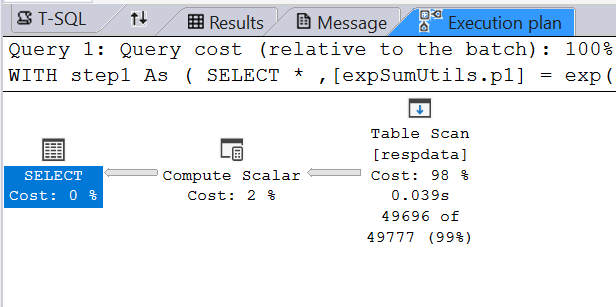
With all three steps combined, we’re still at just one table scan and the same execution plan:
Respondent Filtering
If there exists a universal respondent filter, we’ll want to apply it so that we’re only calculating the individual probabilities for the included respondents. See row 10 highlighted below:
WITH step1 As (
    SELECT
        *
        ,[expSumUtils.p1] = exp(sku1 + size1 + color2 + price1 + price2*0.59)
        ,[expSumUtils.p2] = exp(sku2 + size1 + color3 + price1 + price2*0.59)
        ,[expSumUtils.p3] = exp(sku3 + size1 + color1 + price1 + price2*0.19)
        ,[expSumUtils.p4] = exp(sku4 + size2 + color3 + price1)
        ,[expSumUtils.p5] = exp(sku5 + size2 + color3 + price1 + price2*0.59)
    FROM respdata
    WHERE gender=1
)
,step2 AS (
    SELECT
        *
        ,[expSumUtils.__sum] =
            [expSumUtils.p1] +
            [expSumUtils.p2] +
            [expSumUtils.p3] +
            [expSumUtils.p4] +
            [expSumUtils.p5]
    FROM step1
)
,step3 AS (
    SELECT
        *
        ,[iProb.p1] = [expSumUtils.p1] / [expSumUtils.__sum]
        ,[iProb.p2] = [expSumUtils.p2] / [expSumUtils.__sum]
        ,[iProb.p3] = [expSumUtils.p3] / [expSumUtils.__sum]
        ,[iProb.p4] = [expSumUtils.p4] / [expSumUtils.__sum]
        ,[iProb.p5] = [expSumUtils.p5] / [expSumUtils.__sum]
    from step2
)
select * from step3
This is where an Index will come in handy and improve record seek time.
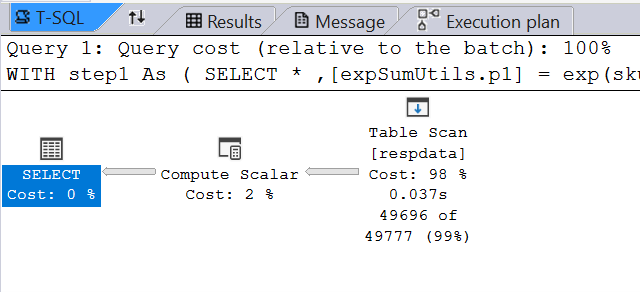
Without index:
CREATE INDEX idx_gender ON respdata (gender)
INCLUDE (
    [respid], [sku1], [sku2], [sku3], [sku4], [sku5],
    [size1], [size2], [color1], [color2], [color3],
    [price1], [price2], [region], [group1], [group2]
)
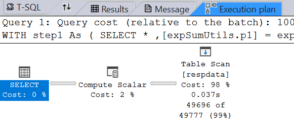
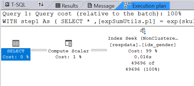
With index (improved speed):
I’m removing the index and respondent filter for the rest of the documentation.
Step 4: Aggregate iProbs
We calculate the share as an average of the individual probabilities.
,aggregate1 AS (
    SELECT
        [share.p1] = avg([iProb.p1]),
        [share.p2] = avg([iProb.p2]),
        [share.p3] = avg([iProb.p3]),
        [share.p4] = avg([iProb.p4]),
        [share.p5] = avg([iProb.p5]),
        [n] = count(*)
    FROM step3
)
The result is a single row with a share for each product:

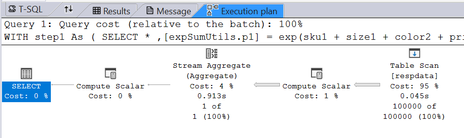
The query execution now includes an aggregation stream.
Step 4 (Alt): Aggregation with comparison groups
If comparison groups are present, we include them in aggregation.
,aggregate1 AS (
    SELECT
        -- group1
        [share.p1.group1] = avg(CASE when group1=1 then [iProb.p1] else null END),
        [share.p2.group1] = avg(CASE when group1=1 then [iProb.p2] else null END),
        [share.p3.group1] = avg(CASE when group1=1 then [iProb.p3] else null END),
        [share.p4.group1] = avg(CASE when group1=1 then [iProb.p4] else null END),
        [share.p5.group1] = avg(CASE when group1=1 then [iProb.p5] else null END),
        [n.group1] = count(CASE when group1=1 then 1 else null end),

        -- group2
        [share.p1.group2] = avg(CASE when group2=1 then [iProb.p1] else null END),
        [share.p2.group2] = avg(CASE when group2=1 then [iProb.p2] else null END),
        [share.p3.group2] = avg(CASE when group2=1 then [iProb.p3] else null END),
        [share.p4.group2] = avg(CASE when group2=1 then [iProb.p4] else null END),
        [share.p5.group2] = avg(CASE when group2=1 then [iProb.p5] else null END),
        [n.group2] = count(CASE when group2=1 then 1 else null end)
    FROM step3
)
Another way to break the results out by group is to use the GROUP BY expression. Sometimes I’ll also use a hybrid of GROUP BY and the CASE statements above. But for this explanation I’m keeping things simple.
The result is still a single row, but with a share of each product by each group.

The execution plan is still the same but probably uses a bit more memory and takes a little longer: